Geometric Meaning of Vector-Scalar Multiplication

In this article, you’ll learn why numbers are called scalars in linear algebra and understand the geometric interpretation of addition and vector-scalar multiplication.

Source Code → https://github.com/MrSheerluck/linear-algebra/tree/main/vectors/vector-scalar-multiplication

What is a Scalar?

Scalar is just a number in linear algebra and they are generally denoted as

\(\alpha, \beta, \lambda\)

(these are pronounced as alpha, beta and lambda respectively).

Vector Scalar Multiplication

A vector scalar multiplication is denoted as:

\(\lambda \vec{v}\)

This means that a scalar multiplies with a vector.

To give you a numeric example:

Let’s take a vector and a scalar

\(\vec{v} =\begin{bmatrix}2 \\-1 \\3\end{bmatrix},\quad\lambda = 4\)

Now, lets multiply both these two

\(4\vec{v}=4\begin{bmatrix}2 \\-1 \\3\end{bmatrix}=\begin{bmatrix}8 \\-4 \\12\end{bmatrix} \)

You just need to multiply each element of the vector with the scalar and you’ll get your resultant vector.

ok, now that you understood the algebraic way of vector-scalar multiplication, lets now understand what it truly means geometrically.

What Exactly Happens When we Multiply a Scalar with a Vector?

\(\vec{w} = \lambda \vec{v}\)

The geometric understanding of vector-scalar multiplication is to stretch or shrink the vector by the amount specified by the scalar and this doesn’t change the direction of the vector.

Lets take some examples:

As you can see in the video, at first we have a vector

\(\vec{v} = (2,1)\)

then we multiplied that with “2” and it becomes

\(2\vec{v}=(4,2)\)

and then we kept multiplying that by 2 and so on.

Note that, it only scaled up and never changed the direction of that vector.

One more thing, it’ll only scale up when:

\(\lambda > 1\)

.

Another example where the scalar will shrink the vector:

If

\(\lambda \in (0,1)\)

(if lambda value is greater than 0 and less than 1), then the scalar will shrink the vector but it won’t change the length.

There’s another case where

\(\lambda < 1\)

, I’m not going to cover this case here as it’ll confuse you and we will cover it later after learning a concept called subspace. Till then don’t worry about it.

Ok, now lets do this in python and then we will wrap up.

Vector-Scalar Multiplication in Python

First, lets import our usual packages:

import numpy as np
import matplotlib.pyplot as plt
from mpl_toolkits.mplot3d import Axes3D

# vector and scalar
v1 = np.array([ 3, -1 ])
l  = 4
v1m = v1*l # scalar-modulated

# plot them
plt.plot([0, v1[0]],[0, v1[1]],'b',label='$v_1$')
plt.plot([0, v1m[0]],[0, v1m[1]],'r:',label='$\\lambda v_1$')

plt.legend()
plt.axis('square')
axlim = max([max(abs(v1)),max(abs(v1m))])*1.5 # dynamic axis lim
plt.axis((-axlim,axlim,-axlim,axlim))
plt.grid()
plt.show()

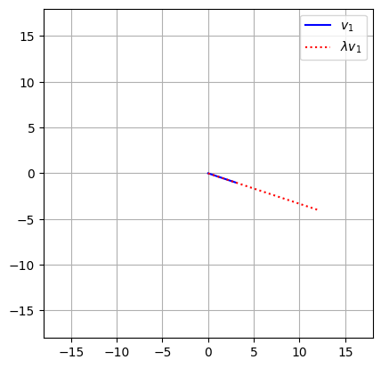
We define our vector v1 as (3, -1) and scalar l as 4. Multiplying them with v1*l gives us the scaled vector (12, -4).

We plot both vectors from the origin - the original v1 in blue and the scaled version in red dotted line.

The axis(’square’) keeps equal scaling on both axes, while axlim dynamically adjusts the plot limits based on the larger vector.

The result clearly shows the vector stretched by a factor of 4 in the same direction.

I hope you learned something interesting especially through the geometric interpretation of vector-scalar multiplication. In the next one, we will learn about vector-vector multiplication a.k.a the dot product. I’ll see you next time, GoodBye!